Software Cost Estimation
Estimating Software cost is an art. Software Sizing is important since the accuracy of the Software Project Estimation depends on –
- the extend to which the planner has properly estimated the size of the project to be built
- ability to translate the estimated product size (in terms of LOC or FP) into human effort, calendar time and dollars.
Based on the nature of the software, software process and team culture there are various approaches to estimating software. We can broadly classify Software Cost estimation techniques into two – Traditional and Agile. We will see both in detail.
A. Traditional Estimation Techniques
Traditional software sizing and estimating techniques are used for software project estimation mainly in terms of cost and effort. There are two broad categories of traditional software sizing and estimation namely – Empirical and Decomposition methods as shown below –
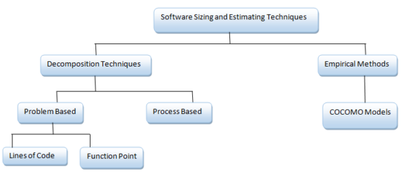
Decomposition based software project estimation depend on the Lines of Code (LOC) value or Function Point (FP) value. This kind of software estimation involves decomposing the Software into individual components and assessing the LOC or FP required to complete each unit. Two famous estimation techniques that uses this sizing technique are Delphi (Expert Judgement based approach) and the Work break down approach (Top down approach). We shall see both of these decomposition based techniques as explained in sections 1 and 2 below. Empirical method is based on bottom up approach where the software cost and effort is arrived at using a table of empirical values for various types of Software. We will see an example Empirical model called COCOMO model in section 3.
1. Delphi Cost estimation or Top Down approach
Delphi cost estimation is an expert judgement based method of software cost estimation. Two of the Delphi methods for software cost estimation is explained below.
Method 1: In this method, the members of the estimation team do not discuss each other about the estimates and makes the estimates anonymously, but could communicate with the coordinator. The methods is as follows –
- The coordinator supplies the system definition/specification to each of the estimator and supplies a form to it fill it up
- The estimator evaluates the system definition/specification and submits to the coordinator
- The coordinator evaluates them and prepares a summary of those estimates and supplies the summary and any story points pointed out by any of the estimators to each of the estimators
- The estimators now again prepares individual estimations and submit the estimation
- The above process is repeated until a group consensus is reached.
Method 2: In this method, the estimators are allowed to communicate with the coordinator and with one another, but prepare estimations anonymously. The process is same as above, the only difference is that estimators are allowed to discuss on the estimation summaries and other issues brought up with the estimator and with one another.
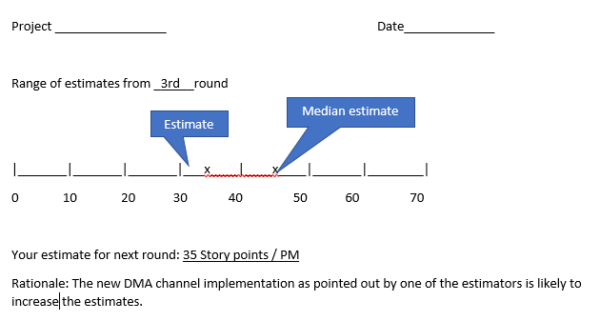
A sample estimation form used for Delphi cost estimation is as shown below
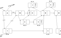
2. Work Break Down Structure or Bottom up approach
A work breakdown structure is a hierarchical chart that accounts for the individual parts of a system. A product work break down structure shows how the software product may be decomposed top-down and it shows the estimation and interconnections between the various component parts as shown below –
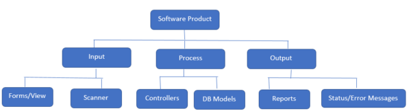
Once we break down the tasks bottom up, costs are estimated by assigning cost to each individual component in the chart and summing the costs.
3. Algorithmic (Empirical) Cost Model – COCOMO (Constructive Cost Model) Model
Algorithmic or Empirical cost models follow the bottom-up method of software cost estimation. Such models follow systematic steps to arrive at the software product cost. COCOMO or constructive cost model introduced by Boehm. COCOMO may be applied to the following types of software products.
Organic application products which involves a small group of highly experienced people working in less rigid environments.
Semidetached products which involves a group of mixed experienced people working on rigid or less rigid analysis and design requirements.
Embedded or system level products involve a set of hardware, software, interfaces.
According to level of product complexity, Boehm introduced 3 types of COCOMOs – Basic, Intermediate and Advanced COCOMO.
3.1 Basic COCOMO
Basic COCOMO is based on the size of the software product in terms of KLOC (kilo lines of code). Basic COCOMO uses the following table to compute the coefficient values ab, bb, cb, db used in the estimation formula
ab bb cb db
Organic 2.4 1.05 2.5 0.38
Semidetached 3 1.12 2.5 0.35
Embedded 3.6 1.2 2.5 0.32
Now, given the total KLOC for the softwareproduct, we calculate the total effort in person month as –
E = ab(KLOC)bb ———————–(1)
and total development time as,
D = cb(E)db ———————–(2)
Now, considering rate of dollar x/Programmer month, we get –
Total estimated project cost = E*x
Example Scenario: Consider a typical line testing software used in telecom having the following sub-systems and related lines of code-
- User interface and control features (1,500)
- Database related (1,000)
- Line testing interface (2000)
- Data communication module (2000)
- Peripheral control (1000)
- Output and reporting features (1000)
- Application Processing (1500)
Total KLOC = 10
Now, since the line testing software can be considered as an embedded software, we may use the coefficient values correspondingly from the above table. Thus, we get –
Total Effort, E = ab(KLOC)bb
= 3.6(10)1.2
= 57.06 programmer months
Total Development time, D = cb(E)db
= 2.5(57.06)0.32
= 9.12 months
Total persons needed for the project = 57.06 / 9.12 = 6.25 ~ 7 persons
Now, considering a rate of $6000 per programmer month,
Estimated project cost = E * 6000 = 57.06 * 6000 = $342,360
3.2 Intermediate COCOMO
Intermediate COCOMO considers certain cost drivers and introduces an effort adjustment factor on the computed effort & cost in terms of KLOC. Cost drivers and their attributes are as shown below –
| Cost Driver | Cost Driver attribute (15) |
| Product | (PR) Product Reliability (DS) Database Size (PC) Product Complexity |
| Computer | (ETC) Execution Time Constraints (MSC) Main Storage COnstraint (VMV) Virtual Machine volatility (CTAT) Computer Turn Around Time |
| Personal | (AC) Analyst Capability (AE) Application Experience (PC) Programmer Capability (PLE) Programmer Language Experience (VME) Virtual Machine Experience |
| Project | (MPP) Modern Programming Practices (UST) Use of third party software tools (RTS) Required Time Schedule |
Now, the above cost driven attributes are given a value from 0.75 to 1.65 as following scale indicates-
Very Low Low Nominal High Very High Extremely High
0.75 0.88 1 1.15 1.4 1.65
The assessed values of the above cost driven attributes are now multiplied to get an Effort Adjustment Factor (EAF) whose value lie in range 0.9 – 1.4. The various coefficient values are as follows –
ai bi ci di
Organic 3.2 1.05 2.5 0.38
Semidetached 3.0 1.12 2.5 0.35
Embedded 2.8 1.2 2.5 0.32
Thus we compute various estimated values as,
E = ai(KLOC)bi * EAF (Person months)———————–(1)
and total development time as,
D = cb(E)db ———————–(2)
At a rate of $x/person month,
Estimated cost = E*x (in dollars)
Example Scenario: For the example introduced in Basic COCOMO model above, we shall subjectively assess the various cost driver attribute values as follows –
| CDA | Value |
| PR | 1 |
| DS | 0.88 |
| PC | 1.22 |
| ETC | 1.01 |
| MSC | 1 |
| VMV | 1.21 |
| CTAT | 1 |
| AC | 0.88 |
| AE | 1.1 |
| PC | 0.88 |
| PLE | 1.2 |
| VME | 1.11 |
| MPP | 1 |
| UST | 0.86 |
| RTS | 1 |
Effort adjustment factor (EAF) = 1 * 0.88 * 1.11 * …. * 1 = 1.28
Total Effort, E = ai(KLOC)bi * 1.28
= 2.8(10)1.2 * 1.28
= 73.04 programmer months
Total Development time, D = cb(E)db
= 2.5(73.04)0.32
= 9.8 months
Total persons needed for the project = 73.04 / 9.8 = 7.45 ~ 8 persons
Now, considering a rate of $6000 per programmer month,
Estimated project cost = E * 6000 = 73.04 * 6000 = $438,240
3.3 Advanced COCOMO
Advanced COCOMO further considers the cost driver impact on each software sub system and functions.
Other related articles that you might be interested in –
1. Factors Affecting Software Cost
2. Programming Team Structures
3. Software Development Team Structures
4. Factors Affecting Software Quality and Developer Productivity
5. Managerial Issues of Software Engineering
6. Connecting Traditional Water Fall Software Life Cycle Model with Agile Models
8. Software Engineering then and now
Working as team, not always good in an organization